Import standard modules:
import numpy as np
import matplotlib.pyplot as plt
%matplotlib inline
from IPython.display import HTML
HTML('../style/course.css') #apply general CSS
2.10 Linear Algebra
In the sections that follow we will be studying vectors and matrices. We use vectors and matrices quite frequently in radio interferometry which is why it is quite important to have some familiarity with them.
2.10.1 Vectors
Definition: An $n$-dimensional column vector ${\bf v } \in\mathbb{C}^{n\times 1}$ is an ordered collection of $n$-complex numbers, i.e. $v_1,v_2,....v_n$; stacked in the following manner:
\begin{equation} {\bf v } = \begin{pmatrix} v_1\\ v_2\\ \vdots\\ v_n \end{pmatrix}. \end{equation}An $n$-dimensional row vector ${\bf u}^T \in\mathbb{C}^{1\times n}$ is an ordered collection of $n$-complex numbers, i.e. $u_1,u_2,....u_n$; stacked in the following manner:
\begin{equation} {\bf u }^T=(u_1,u_2,....u_n). \end{equation}Note that, with this notation, a vector $\bf{v}$ is always assumed to be a column vector and we explicitly use a superscipt $T$ to indicate that a row vector is the transpose of a vector. Thus it should be understood that the notation ${\bf{v}}\in\mathbb{C}^{n}$ denotes a column vector.
2.10.1.1 Vector Products
Suppose that ${\bf{u}},{\bf{v}}\in \mathbb{C}^{n}$. The following vector products are often used in radio interferometry:
Hermitian inner product:
The Hermitian inner product of ${\bf{u}}$ and ${\bf{v}}$ is given by
\begin{equation} {\bf{u}}\cdot{\bf{v}} = {\bf u}^H {\bf v} = \sum_{k=1}^n u_i^*v_i, \end{equation}
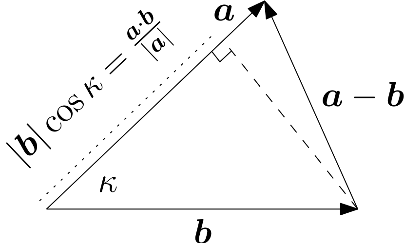
where the superscript $H$ denotes the Hermitian transpose (see below). Recall that the inner product of a real vector ${\bf b} \in \mathbb{R}^n$ with a real unit vector $\hat{{\bf a}} \in \mathbb{R}^n$ (where $\hat{{\bf a}} = {\bf \frac{a}{|a|}}$) gives the component of ${\bf b}$ in the direction defined by $\hat{{\bf a}}$. The inner product on real vectors is sometimes refered to as the dot product and we say that it projects ${\bf b}$ onto $\hat{{\bf a}}$. Explicitly we have
\begin{equation} {\bf b }\cdot{\bf \hat{a}} = |{\bf b}| \ |{\bf \hat{a}}| \cos(\kappa) = |{\bf b}|\cos(\theta), \end{equation}
where $|\cdot|$ denotes the magnitude of a vector and $\kappa$ is the acute angle between $\hat{{\bf a}}$ and ${\bf b }$. This is illustrated in Fig. 2.10.1 ⤵
Outer Product:
The outer product of ${\bf{u}}$ and ${\bf{v}}$ is given by
\begin{equation} {\bf u} {\bf v} = {\bf u }{\bf v}^H, \quad \rightarrow \quad {(\bf{u}}{\bf{v})}_{ij} = u_iv_j^* \end{equation}
We may also assign a geometric meaning to the outer product. In the case where both vectors are unit vectors viz. ${\bf \hat{u}}$ and ${\bf \hat{v}}$, we may think of the outer product as an operator which acts on an arbitrary vector ${\bf x}$ to produce
\begin{equation} ({\bf \hat{u}} * {\bf \hat{v}}) {\bf x} = {\bf \hat{u} }{\bf \hat{v}}^H {\bf x} = {\bf \hat{u} }({\bf \hat{v}}\cdot {\bf x}). \end{equation}
Thus this operator finds the component of ${\bf x}$ along the direction of ${\bf \hat{v}}$ and points it in the direction of ${\bf \hat{u}}$.
2.10.2 Matrices
Definition: A matrix ${\bf{A}}\in \mathbb{C}^{m\times n}$ is defined as an ordered rectangular array of complex numbers, i.e. \begin{equation} {\bf{A}} = \begin{pmatrix} a{11}&a{12}&\dots& a{1n}\ a{21}&a{22}&\dots &a{2n}\ \vdots&\vdots&\ddots &\vdots\ a{m1}&a{m2}&\dots &a_{mn} \end{pmatrix} \end{equation}
If $m=n$, then ${\bf{A}}$ is a square matrix. Note that the first index is used to label the row number and the second the column number.
2.10.2.1 Basic Matrix Operations and Properties
The traspose of ${\bf{A}}\in \mathbb{C}^{m\times n}$, denoted by ${\bf{A}}^T$ is given by \begin{equation} {\bf{A}}^T{ij} = a{ji}, \end{equation} i.e. the transpose operation interchanges the rows and columns of the matrix.
The complex conjugate of ${\bf{A}}\in \mathbb{C}^{m\times n}$, denoted by ${\bf{A}}^*$ is given by \begin{equation} {\bf{A}}^{ij} = a{ij}^. \end{equation}
The Hermitian tranpose of ${\bf{A}}\in \mathbb{C}^{m\times n}$, denoted by ${\bf{A}}^H$ is given by \begin{equation} {\bf{A}}^H{ij} = a{ji}^, \end{equation} i.e. the Hermitian transpose is the conjugate of the transposed matrix ${\bf A}^H = ({\bf A}^T)^$.
The vectorization of matrix ${\bf{A}}\in \mathbb{C}^{m\times n}$, denoted by vec$({\bf{A}})$, is the $mn \times 1$ column vector obtained by stacking the columns of the matrix ${\bf{A}}$ on top of one another: \begin{equation} \mathrm{vec}({\bf{A}}) = [a{11}, \ldots, a{m1}, a{12}, \ldots, a{m2}, \ldots, a{1n},\ldots, a{mn}]^T \end{equation} The inverse operation of of vec$({\bf{A}})$ is denoted by vec$^{-1}({\bf{A}})$. We will refer to this operation as the matrization. This should not be confused with matricization which is the generalisation of vectorisation to higher order tensors.
We use diag$(\bf{u})$ to denote a matrix whose diagonal is equal to $\bf{u}$, while all its other entries are set to zero. Conversely, when applied to a matrix ${\bf A}$, the notation diag$({\bf A})$ refers to the vector formed by extracting only the diagonal elements of ${\bf A}$.
A square matrix ${\bf{A}}\in \mathbb{C}^{m\times m}$ is said to be:
- Invertible if there exists a matrix ${\bf{B}}\in \mathbb{C}^{m\times m}$ such that: \begin{equation} {\bf{B}}{\bf{A}} = {\bf{A}}{\bf{B}} ={\bf{I}}. \end{equation} We denote the inverse of ${\bf{A}}$ with ${\bf{A}}^{-1}$.
- Hermitian if ${\bf{A}} = {\bf{A}}^H$.
- (Special-) Orthogonal if ${\bf AA}^T = I \rightarrow {\bf{A}}^{-1} = {\bf{A}}^T$.
- (Special-) Unitary if ${\bf A A}^H = I \rightarrow {\bf{A}}^{-1} = {\bf{A}}^H$.
2.10.2.2 Matrix Products
There are a few matrix products which are commonly used in radio interferometry. We define the most frequently used matrix products below (also see Hadamard, Khatri-Rao, Kronecker and other matrix products ⤴ however be aware that our notation differs from the notation used there).
We assume below that ${\bf{A}},{\bf{C}}\in\mathbb{C}^{m\times n}$, ${\bf{B}}\in\mathbb{C}^{p\times q}$ and ${\bf{D}}\in\mathbb{C}^{n\times r}$. Sometimes it will be necessary to partition the matrices into sub-matrices. We will use boldface subscripts to refer to sub-matrices. For example, the notation ${\bf{A}}_{\bf ij}$ refers to the sub-matrix ${\bf{A}}_{\bf ij}\in\mathbb{C}^{m_i\times n_j}$ of the matrix ${\bf A}$. Thus the boldface indices ${\bf i}$ and ${\bf j}$ are themselves lists of indices of length $m_i$ and $n_j$, respectively. Similarly, the notation ${\bf{B}}_{\bf kl}$ refers to the sub-matrix ${\bf{B}}_{\bf kl}\in\mathbb{C}^{p_k\times q_l}$ of the matrix ${\bf B}$ and this time the boldface indices ${\bf k}$ and ${\bf l}$ are lists of length $p_k$ and $q_l$ respectively. The meaning of this notation will become clearer in the examples below. For now keep in mind that the boldface indices are lists whose elements do not necessarily need to start counting from one (see the definition of the Kronecker product below). Moreover $\sum m_i = m, \sum n_j = n, \sum p_k = p$ and $\sum q_l = q$. We can now define the following matrix products:
Matrix Product The matrix product of ${\bf{A}}$ and ${\bf{D}}$, denoted ${\bf{A}}{\bf{D}}$, is of order $m\times r$. The $ij$-th element of the matrix product is given by
\begin{equation} ({\bf{A}} {\bf{D}}){ij} = \sum^m{k=1} a{ik}b{kj}. \end{equation}
Note that the number of columns of ${\bf{A}}$ must be equal to the number of rows of ${\bf{D}}$ for this product to exist.
Hadamard Product
The Hadamard product of ${\bf{A}}$ and ${\bf{C}}$, denoted ${\bf{A}}\odot{\bf{C}}$, is the element-wise product of ${\bf{A}}$ and ${\bf{C}}$ i.e.
\begin{equation} {(\bf{A}} \odot {\bf{C}}){ij} = a{ij}c_{ij}. \end{equation}
Note that ${\bf{A}}$ and ${\bf{C}}$ must be of the same order for this product to exist and that the resulting matrix will be of the same order as both ${\bf A}$ and ${\bf C}$. We may also define the Hadamard or elementwise inverse of a matrix ${\bf A}$. The $ij-$th element of the Haramard inverse is given by \begin{equation} (A^{\odot -1}){ij} = \frac{1}{a{ij}} \end{equation}
Kronecker Product
The Kronecker product of ${\bf A}$ and ${\bf B}$, denoted ${\bf A} \otimes {\bf B}$, multiplies every element of ${\bf A}$ with every element of ${\bf B}$ and arranges the result in a matrix of the following form
\begin{equation} {\bf{A}} \otimes {\bf{B}} = \left(\begin{array}{ccc}a{11}{\bf B} & a{12}{\bf B} & \cdots & a{1n}{\bf B} \ a{21}{\bf B} & a{22}{\bf B} & \cdots & a{2n}{\bf B} \ \cdot & \cdot & \cdot & \cdot \ a{m1}{\bf B} & a{m2}{\bf B} & \cdots & a_{mn}{\bf B} \end{array}\right). \end{equation}
Note that the resulting matrix is of order $mp\times nq$. Using the boldface indices introduced above we may also write this as
\begin{equation} ({\bf{A}} \otimes {\bf{B}}){\bf ij} = a{ij}{\bf{B}}. \end{equation}
Note that the boldface indices ${\bf ij}$ always correspond to the indices of the element $a_{ij}$ of the original matrix ${\bf A}$. If we think of the result of the Kronecker product as the matrix ${\bf Q} = {\bf{A}} \otimes {\bf{B}}$ where ${\bf Q} \in \mathbb{C}^{mp\times nq}$, then
\begin{equation} ({\bf{A}} \otimes {\bf{B}}){\bf ij} = {\bf Q}{(ip+1):(i+1)p \ , \ (jq+1):(j+1)q} \ . \end{equation}
In other words the boldface index ${\bf i}$ is a list of indices starting at $ip+1$ and ending at $(i+1)p$ and similarly ${\bf j}$ is a list of indices starting at $jq+1$ and ending at $(j+1)q$. This notation can be difficult to get used to but it will be useful in practical implementations involving the Kronecker product.
Khatri-Rao Product
The Khatri-Rao product, denoted ${\bf{A}} \oplus {\bf{B}}$, can be defined in terms of the Kronecker product. Operationally the Khatri-Rao product of ${\bf{A}}$ and ${\bf{B}}$ is the same as the Kronecker product of each row of ${\bf{A}}$ with the corresponding row of ${\bf{B}}$. We will use the notation ${\bf A}_{i,:}$ to denote the $i-$th row of the matrix ${\bf A}$ (i.e. ${\bf A}_{i,:} = {\bf A}_{i,1:n}$) and similarly ${\bf B}_{k,:}$ denotes the $k-$th row of ${\bf B}$. The Khatri-Rao product can then be defined as
\begin{equation} {\bf{A}} \oplus {\bf{B}} = \left(\begin{array}{c} {\bf A}{1,:} \otimes {\bf B}{1,:} \ {\bf A}{2,:} \otimes {\bf B}{2,:} \ \cdot \ {\bf A}{n,:} \otimes {\bf B}{n,:} \end{array} \right). \end{equation}
Note that the matrices ${\bf A}$ and ${\bf B}$ must have the same number of rows for the Khatri-Rao product to be defined and, if ${\bf A} \in \mathbb{C}^{m\times n}$ and ${\bf B} \in \mathbb{C}^{m\times q}$, the result will be of order $m\times nq$. We should point out that a different convention is sometimes used for the Khatri-Rao product. Our convention has been chosen because it is the one that is encountered most frequently in radio-interferometry.
During this course the Kronecker and Khatri-Rao products will mainly be used to convert between the Jones and Mueller formalisms $\S$ 7 ➞.
2.10.2.3 Examples
Consider the vectors ${\bf{u}}=\begin{pmatrix} u_1,u_2,u_3\end{pmatrix}^T$ and ${\bf{v}}=\begin{pmatrix} v_1,v_2,v_3\end{pmatrix}^T$.
Now: \begin{align} {\bf{u}}*{\bf{v}}&= \begin{pmatrix} u_1\u_2\u_3\end{pmatrix}\begin{pmatrix}v_1,v_2,v_3\end{pmatrix}=\begin{pmatrix} u_1v_1&u_1v_2&u_1v_3\ u_2v_1&u_2v_2&u_2v_3\u_3v_1&u_3v_2&u_3v3\end{pmatrix}. \end{align} Consider the matrices \begin{equation} {\bf{A}} = \begin{pmatrix} a{11}&a{12}\a{21}&a{22}\a{31}&a{32}\end{pmatrix} \hspace{0.5cm} \text{and} \hspace{0.5cm} {\bf{B}} = \begin{pmatrix}b{11}&b{12}\b{21}&b{22}\b{31}&b{32}\end{pmatrix}. \end{equation} Now: \begin{align} {\bf{A}} \odot {\bf{B}} &= \begin{pmatrix} a{11}&a{12}\a{21}&a{22}\a{31}&a{32}\end{pmatrix}\odot \begin{pmatrix}b{11}&b{12}\b{21}&b{22}\b{31}&b{32}\end{pmatrix} = \begin{pmatrix} a{11}b{11}&a{12}b{12}\a{21}b{21}&a{22}b{22}\a{31}b{31}&a{32}b{32}\end{pmatrix}\ {\bf{A}} \otimes {\bf{B}} &= \begin{pmatrix} a{11}&a{12}\a{21}&a{22}\a{31}&a{32}\end{pmatrix}\otimes \begin{pmatrix}b{11}&b{12}\b{21}&b{22}\b{31}&b{32}\end{pmatrix} = \begin{pmatrix} a{11}b{11}&a{11}b{12}&a{12}b{11}&a{12}b{12}\a{11}a{21}&a{11}b{22}&a{12}b{21}&a{12}b{22}\a{11}b{31}&a{11}b{32}&a{12}b{31}&a{12}b{32}\a{21}b{11}&a{21}b{12}&a{22}b{11}&a{22}b{12}\a{21}a{21}&a{21}b{22}&a{22}b{21}&a{22}b{22}\a{21}b{31}&a{21}b{33}&a{22}b{33}&a{22}b{32}\a{31}b{11}&a{31}b{12}&a{32}b{11}&a{32}b{12}\a{31}a{21}&a{31}b{22}&a{32}b{21}&a{32}b{22}\a{31}b{31}&a{31}b{32}&a{32}b{31}&a{32}b{32} \end{pmatrix}\ {\bf{A}} \oplus {\bf{B}} &= \begin{pmatrix} a{11}&a{12}\a{21}&a{22}\a{31}&a{32}\end{pmatrix}\oplus \begin{pmatrix}b{11}&b{12}\b{21}&b{22}\b{31}&b{32}\end{pmatrix} = \begin{pmatrix} {\bf A}{1,:} \otimes {\bf B}{1,:} \{\bf A}{2,:} \otimes {\bf B}{2,:} \ {\bf A}{3,:} \otimes {\bf B}{3,:} \end{pmatrix}\ &= \begin{pmatrix} a{11}b{11}&a{11}b{21}&a{12}b{11}&a{12}b{12}\a{21}b{21}&a{21}b{22}&a{22}b{21}&a{22}b{22}\ a{31}b{31}&a{31}b{32}&a{32}b{31}&a{32}b_{32}\end{pmatrix} \end{align}
Ipython implemenations of the above examples are given below:
# Defining the vectors and matrices
u = np.array((3.,4.,1j)) # 3x1 vector
v = np.array((2.,1.,7.)) # 3x1 vector
A = np.array(([3,4],[5,-1],[4,-2j])) #3x2 matrix
B = np.array(([1,-8],[2,3],[6,1-5j])) #3x2 matrix

# Outer product
out_prod = np.outer(u,v)
# Hadamard product
had_prod = A*B
# Kronecker product
kron_prod = np.kron(A,B)
# Khatri-Rao product
kha_prod = np.zeros((3,4),dtype=complex) # create a matrix of order (m x n^2 = 3X4 matrix)
for i in range(len(A[:,0])):
    kha_prod[i,:] = np.kron(A[i,:],B[i,:])

# Printing inputs and products:
print 'u:', u
print 'v:', v
print "\n Outer Product: (%i x %i)\n"%(out_prod.shape), out_prod
print '\n-------------------------------------'
print 'A: (%i x %i)\n'%(A.shape), A
print 'B: (%i x %i)\n'%(B.shape), B
print "\n Hadamard Product: (%i x %i)\n"%(had_prod.shape), had_prod
print "\n Kronecker Product: (%i x %i)\n"%(kron_prod.shape), kron_prod
print "\n Khatri-Rao Product: (%i x %i)\n"%(kha_prod.shape), kha_prod
2.10.2.4 Product Identities
We can establish the following product identities (assuming the matrices and vectors below have the appropriate dimensions):
$({\bf{A}} \oplus {\bf{B}}) \odot ({\bf{C}} \oplus {\bf{D}})=({\bf{A}} \odot {\bf{C}}) \oplus({\bf{B}} \odot {\bf{D}}) $
$({\bf{A}} \otimes {\bf{B}})({\bf{C}} \oplus {\bf{D}}) = {\bf{A}}{\bf{C}} \oplus {\bf{B}}{\bf{D}}$
$({\bf{A}} \oplus {\bf{B}})^H({\bf{C}} \oplus {\bf{D}}) = {\bf{A}}^H{\bf{C}} \odot {\bf{B}}^H {\bf{D}}$
$\text{vec}({\bf{A}}{\bf{X}}{\bf{B}}) = ({\bf{B}}^T \otimes {\bf{A}})\text{vec}({\bf{X}})$
$\text{vec}({\bf{A}}\text{diag}({\bf{x}}){\bf{B}}) = ({\bf{B}}^T \oplus {\bf{A}}){\bf{x}}$
for more information about these identities the reader is referred to Hadamard, Khatri-Rao, Kronecker and other matrix products ⤴ and (Fundamental imaging limits of radio telescope arrays ⤴). Although we will not be making extensive use of these identities (however see $\S$ 7 ➞), they are frequently encountered in radio interferometry literature especially as it pertains to calibration. To gain some fimiliarity with them we will quickly validate identity four with an example. The others can be verified in a similar way.
Consider the two complex $2\times 2$ matrices: \begin{equation} {\bf{J}} = \begin{pmatrix} j{11} &j{12}\ j{21}&j{22}\end{pmatrix} \hspace{0.5cm} \text{and} \hspace{0.5cm} {\bf{C}} = \begin{pmatrix} c{11} &c{12}\ c{21}&c{22}\end{pmatrix}. \end{equation}
Now:
\begin{eqnarray} \text{vec}({\bf{J}}{\bf{C}}{\bf{J}}^H) &=& \begin{pmatrix} j{11} &j{12}\ j{21}&j{22}\end{pmatrix} \begin{pmatrix} c{11} &c{12}\ c{21}&c{22}\end{pmatrix} \begin{pmatrix} j{11}^* &j{21}^\ j_{12}^&j{22}^*\end{pmatrix}\ &=& \begin{pmatrix} j{11}^j{11}c{11} + j_{11}^j{12}c{21} + j{12}^*j{11}c{12} + j{12}^j{12}c{22}\ j_{11}^j{21}c{11} + j{11}^*j{22}c{21} + j{12}^j{21}c{12} + j_{12}^j{22}c{22} \ j{21}^*j{11}c{11} + j{21}^j{12}c{21} + j_{22}^j{11}c{12} + j{22}^*j{12}c{22}\ j{21}^j{21}c{11} + j_{21}^j{22}c{21} + j{22}^*j{21}c{12} + j{22}^j{22}c{22} \end{pmatrix}\ &=& \Bigg[\begin{pmatrix} j_{11}^ &j{12}^*\ j{21}^&j_{22}^\end{pmatrix} \otimes \begin{pmatrix} j{11} &j{12}\j{21}&j{22}\end{pmatrix}\Bigg]\begin{pmatrix}c{11}\c{21}\c{12}\c{22} \end{pmatrix}\ &=& \left ({\bf{J}}^{*} \otimes {\bf{J}}\right ) \text{vec}({\bf{C}})\ &=& \left( \left ({\bf{J}}^{H} \right)^T \otimes {\bf{J}} \right ) \text{vec}({\bf{C}}) \end{eqnarray}
- nice/pretty matrix printing